Introduction
Electron backscatter diffraction (EBSD) is a powerful tool used in materials science and geology for exploring the microstructure and crystal orientations in a wide range of materials and natural samples. Traditionally, EBSD patterns are analyzed using a Hough transform-based approach, where diffraction bands are detected via image processing, and the positions of these detected bands are used to determine the crystal phase and orientation. However, these methods sometimes face challenges with weak, complex, or poor-quality EBSD patterns.
Methods
Spherical indexing has emerged as an exciting advancement in EBSD analysis as an alternative approach to analyzing EBSD patterns. With spherical indexing, experimentally collected EBSD patterns are correlated with a master pattern for a given phase to determine the crystal orientation of each pattern. This master pattern is a precomputed, orientation-independent map of diffraction intensities projected onto a sphere that represents all possible directions for diffracted electrons for a given phase. Typically, the master pattern is generated using a dynamical electron diffraction simulation. This simulation can be computationally intensive and time-consuming, depending on the complexity of the crystal structure and the number of atomic positions within the unit cell of a given phase. To help minimize the impact of this, EDAX OIM Matrix™ includes nearly 300 precalculated master patterns.
There are alternative methods for generating master patterns that require less time than the dynamical diffraction simulations. One method is using a kinematic diffraction model. This model treats the diffraction as a single scattering event and ignores multiple scattering and absorption effects and is therefore faster to compute. While this approach does position the diffraction bands correction in the master pattern, it does not reproduce the intensity variations observed in experimental EBSD patterns.
A second method is to use experimentally collected EBSD patterns to generate a master pattern. With this approach, an EBSD map is collected while saving the patterns. The orientations are measured initially with Hough-based indexing. The best patterns are selected from the dataset, and based on the measured orientation, these patterns are projected onto a master pattern sphere, while applying the known symmetry elements of the phase to cover the correct regions of orientation space for a given phase. Multiple patterns are selected until all of orientation space is represented. This experimental master pattern has the advantage of capturing the actual EBSD pattern intensities observed and can be used to analyze other datasets. This approach can be beneficial when atomic positions within the unit cell are unknown, or if no unique unit cell can be determined.
Materials and results
A good example of applying alternative master patterns is in the analysis of an olivine and orthopyroxene-bearing rock sample. Both olivine and orthopyroxene are mineral groups with a solid solution series varying in magnesium and iron. Typically, a specific mineral is selected from the mineral group, and the information from the mineral is used to generate a master pattern. An example of this for both forsterite and enstatite is shown in Figure 1.
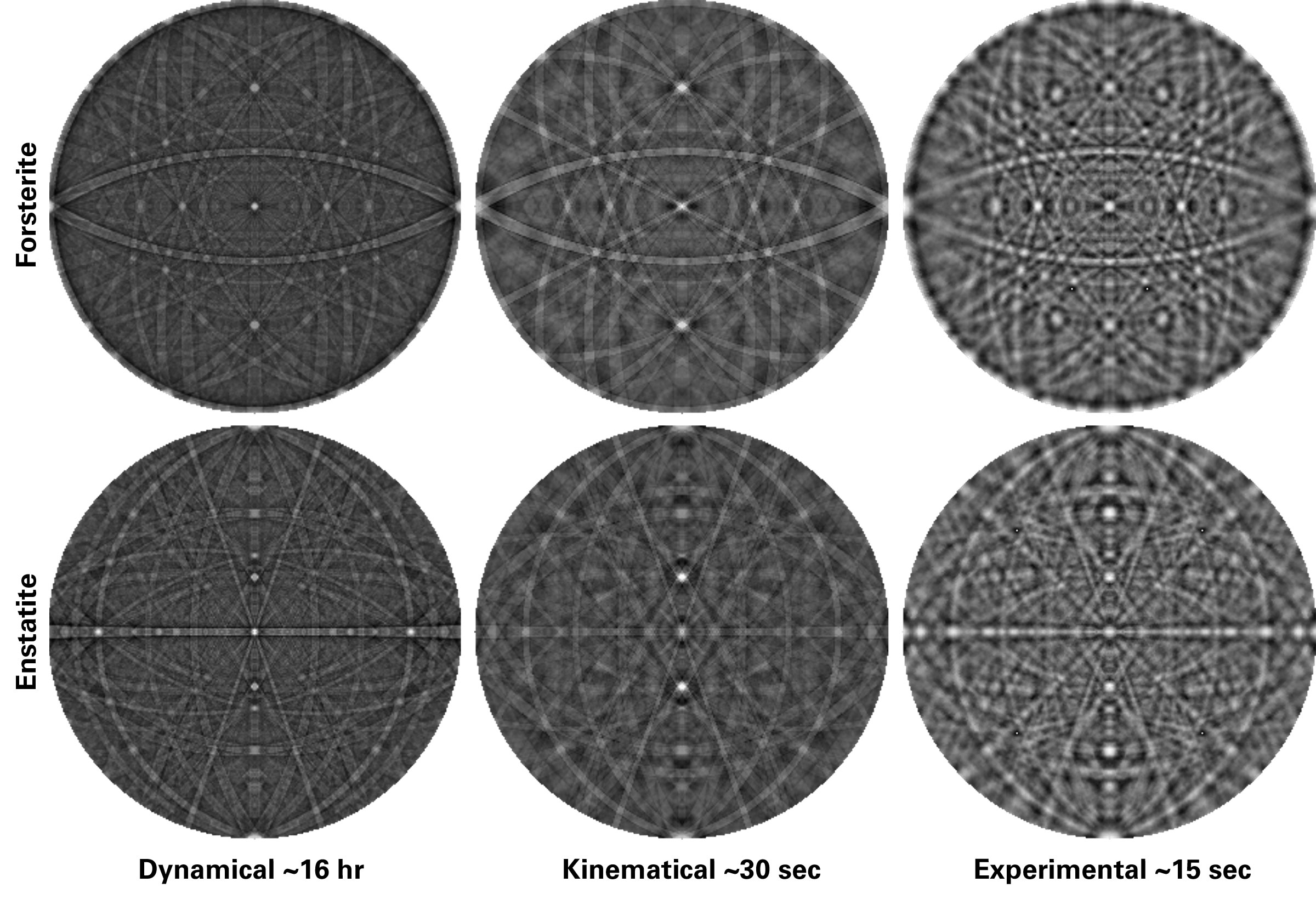
Figure 1. Alternative master patterns for forsterite and enstatite. The dynamical diffraction master patterns took ~16 h, the kinematical approach took ~30 s, and the experimental master patterns were achieved in ~15 s.
These minerals are the magnesium end members of the solid solution ranges for these mineral groups. In this example, the dynamical diffraction master patterns took approximately 16 h to simulate for each phase. In contrast, the kinematical approach took only 30 s, and the experimental master pattern took only 15 s per phase. These time values show a significant reduction in time to achieve a master pattern, which reduces the time to results for spherical indexing performance.
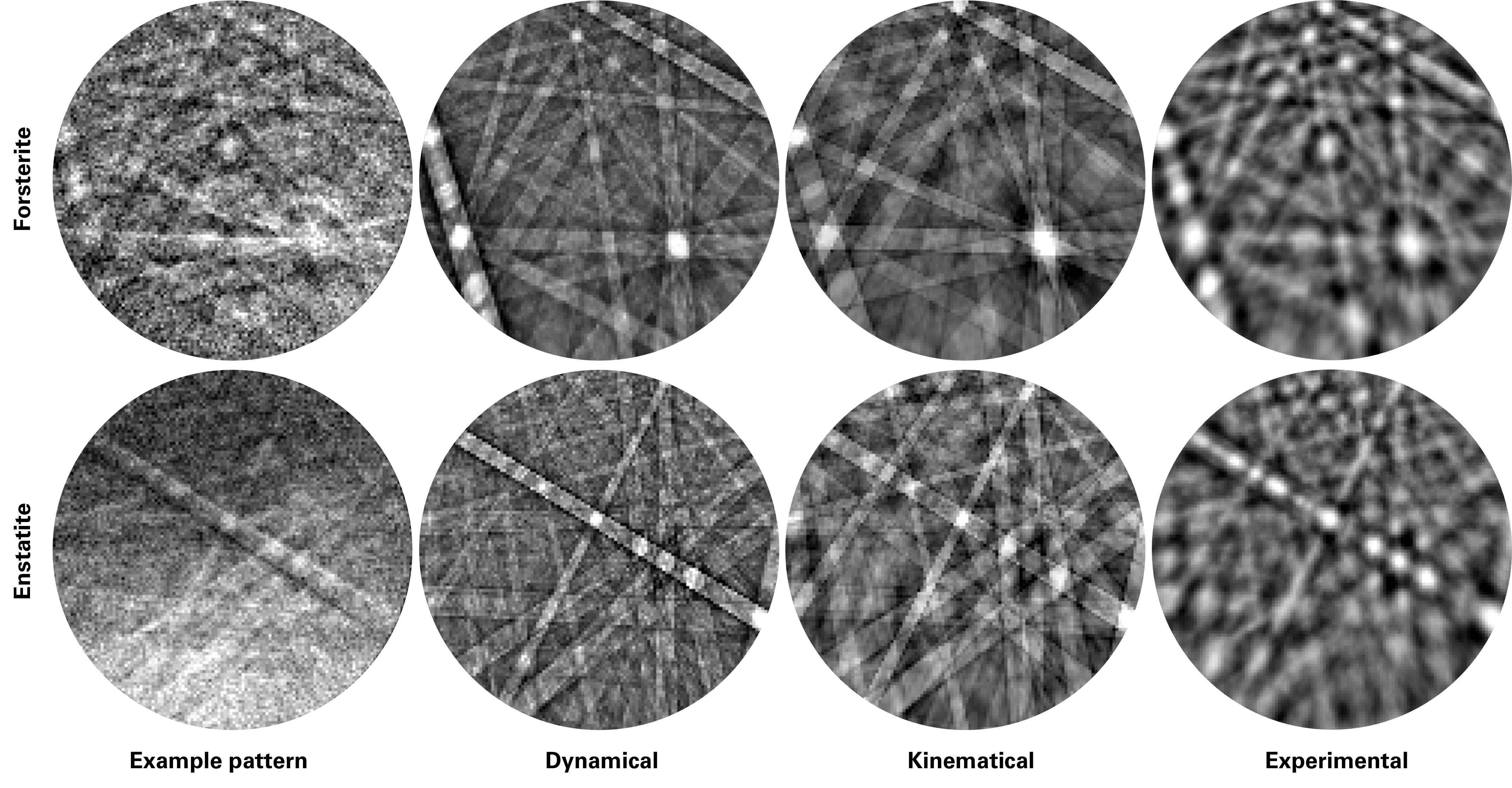
Figure 2. Experimental EBSD pattern from each phase with matching orientations from the three corresponding master patterns shown in Figure 1. This figure shows that the experimental pattern most closely resembles the example pattern, which is to be expected. diffraction band intensities and visible details.
Figure 2 compares a single experimental EBSD pattern from each phase to matching orientations from the three corresponding master patterns shown in Figure 1. This figure shows that the experimental pattern most closely resembles the example pattern, which is to be expected. It also illustrates the differences between the models in terms of the diffraction band intensities and visible details. Often, EBSD pattern quality does not detect these details, depending on sample preparation quality and acquisition conditions.
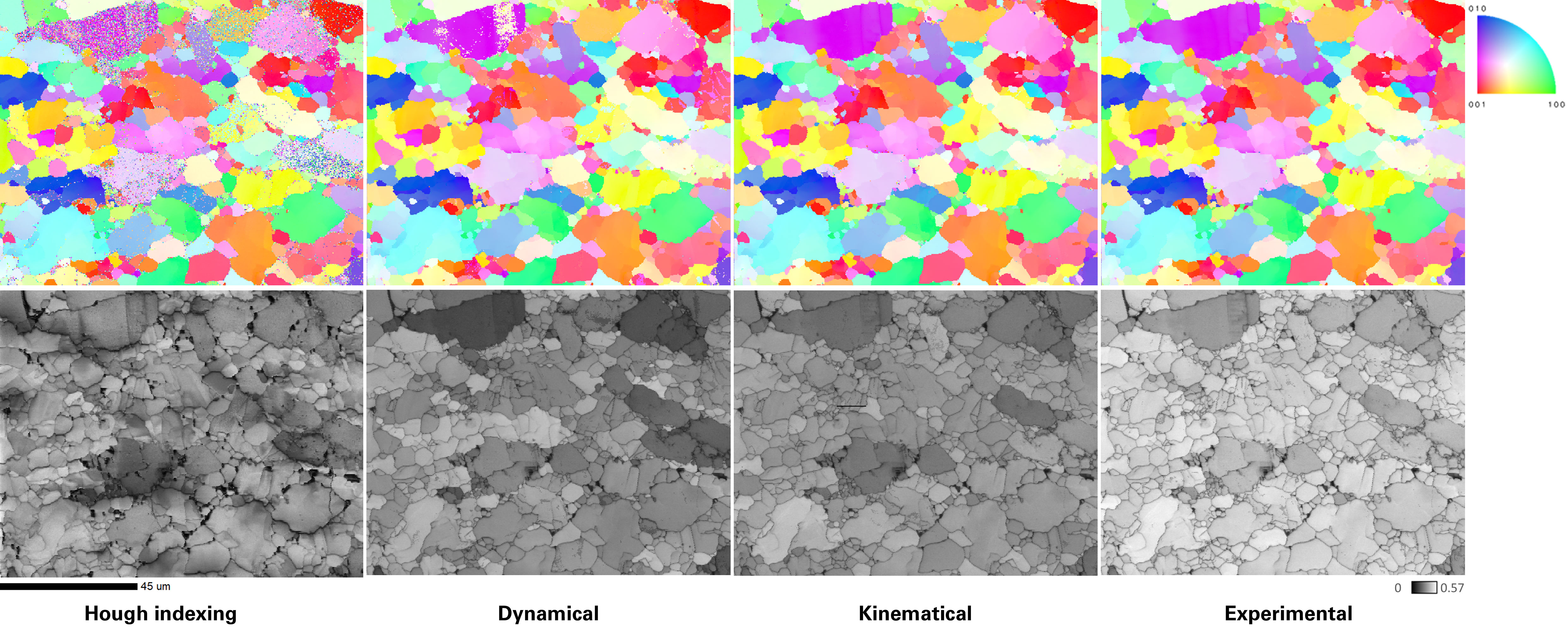
Figure 3. EBSD mapping results using both Hough indexing, and spherical indexing with the three different types of master patterns. IPF maps are shown in the top row and the EBSD quality maps are shown in the bottom row.
Figure 3 shows EBSD mapping results using both Hough indexing and spherical indexing with the three different types of master patterns. This figure depicts both the IPF orientation map relative to the surface normal direction (top), and the EBSD quality map (bottom). For the Hough indexing, the quality metric is the image quality (IQ) value, while for the spherical indexing results, the quality metric is the spherical indexing confidence index (SCI). For the three spherical indexing results, the SCI values are plotted relative to the same grayscale value ranges shown, with lighter shading indicating better correlation.
Examination of the IPF maps shows that some regions are poorly indexed with Hough indexing, and the indexing results significantly improved with spherical indexing. Surprisingly, spherical indexing with the dynamical master pattern has one grain with a region of mis-indexing that is not present with the kinematic or experimental master patterns. This is likely due to the deviation in background processing on this multi-phase sample, and with that an effective pattern contrast difference. Both the kinematic and experimental master patterns provide nearly 100% indexing success rates. Additionally, the experimental master pattern has the highest correlation quality, indicating that using actual experimental patterns to create the master pattern provides better spherical indexing performance. Figure 4 shows the phase map of this area for reference.
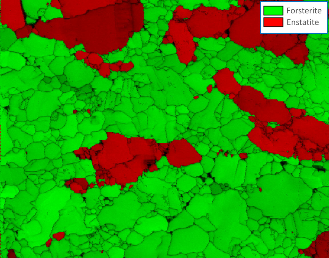
Figure 4. Phase map of the region of analysis.
Conclusion
With spherical indexing, both geologists and materials scientists benefit from faster and more reliable results, making it easier to study everything from engineered alloys to ancient rocks. This technique is quickly becoming a valuable addition to the toolkit, supporting innovative research and everyday investigations in laboratories around the world. Alternative master patterns derived using kinematic diffraction and experimental EBSD patterns provide a faster route to these improved results and are a practical and sometimes preferable option for spherical indexing analysis.